1  Introduction to R

1.1 Introduction

R evolved from the S language, which was first developed by Rick Becker, John Chambers and Allan Wilks. S was created with the following goals in mind:

1. S was conceived as a powerful tool for statistical modelling. It enabled you to specify and fit statistical models to your data, assess the goodness of fit and then display parameter estimates, standard errors and predicted values derived from the model. It provided the means to define and manipulate data. The intent was to provide the user with maximum control over the model-fitting process.
2. S was to be used for data exploration (tabulating, sorting data, drawing plots to look for trends, etc.)
3. It was to be used as a sophisticated calculator to evaluate complex arithmetic expressions, and as a very flexible and general object-oriented programming language to perform more extensive data manipulation.

Later on, S evolved into S-PLUS, which became very costly. Ross Ihaka and Robert Gentleman from the University of Auckland, decided to write a stripped-down version of S, which was R. Five years later, version 1.0.0 of R was released on 29 Feb 2000. As of Dec 2024, the latest version of R is 4.4.2 It is maintained by the (R Core Team 2024).

1.2 Installing R and Rstudio

To download R, go to CRAN, the Comprehensive R Archive Network, download the version for your operating system and install it.

A new major version is released once a year, and there are 2 - 3 minor releases each year. Upgrading is painful, but it gets worse if you wait to upgrade.

Important

For our class, please ensure that you have version 4.4.1 or later. Functions in older versions work differently, so you might face problems or differences with some of the codes in the notes.

Figure 1.1: Base R

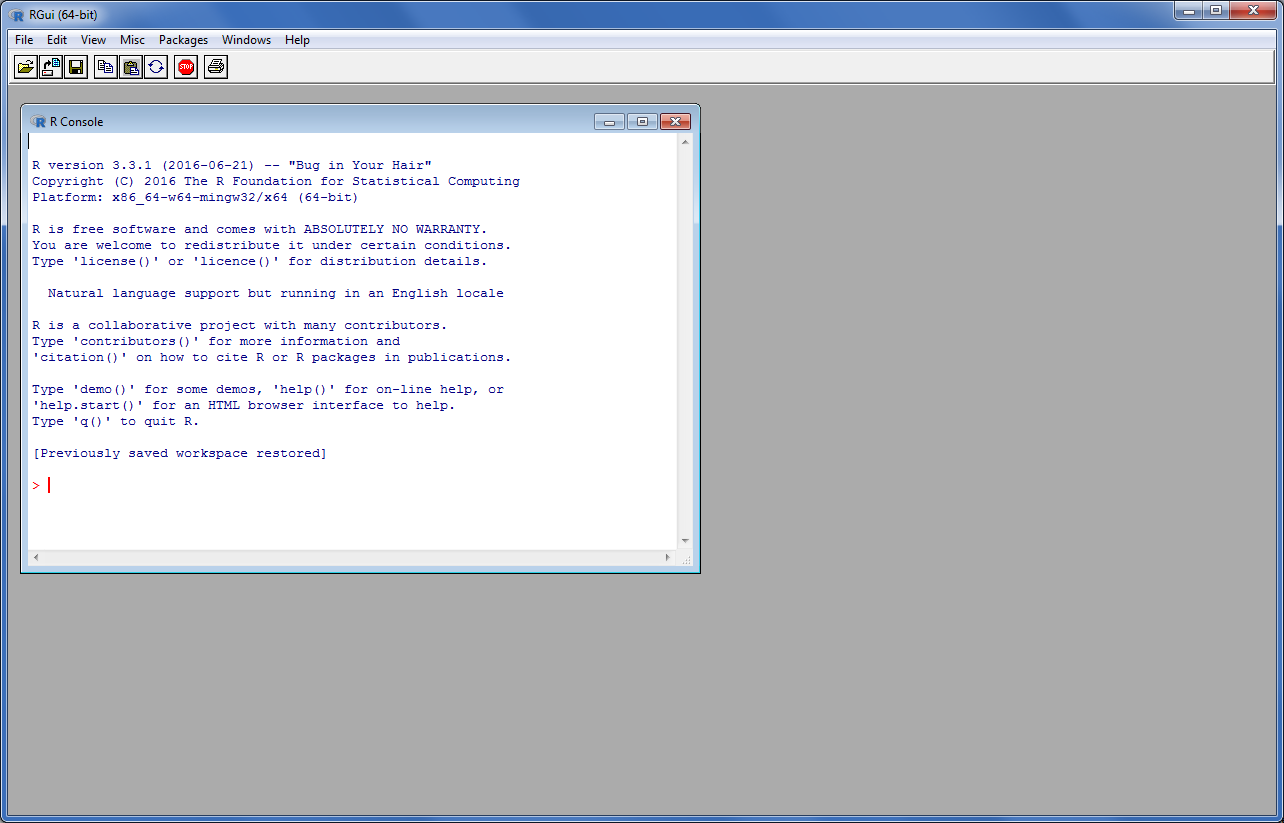
After installing, you can start using R straightaway. However, the basic GUI is not very user-friendly, as you can see from Figure 1.1. Instead of using the basic GUI for R, we are going to use RStudio. RStudio is an Integrated Development Environment (IDE) for R. It provides several features that base R does not, including:

• A history of previous plots made.
• The ability to browse the objects in our workspace more easily.

The installation file for RStudio can be obtained from this URL. It is updated a couple of times a year. Make sure you have at least version 2024.09.x for our course.

Figure 1.2: Rstudio interface

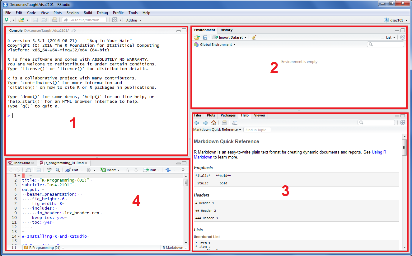
Here’s a quick orientation of the panels in Rstudio, with reference to Figure 1.2.

• Panel 1 is the .
  • This is where you type R commands.
  • The output from these commands or functions will also be seen here.
  • Use the \(\uparrow\) key to scroll through previously entered commands.
• Panel 2 contains the History and Environment tabs.
  • The History tab displays all commands that have been previously entered in the current session.
  • These commands can be sent directly to the source code panel or the console panel.
  • The Environment tab in this panel has a list of items that have been created in the current session.
• Panel 3 contains the Files, Plots and Help tabs.
  • The Files tab contains a directory structure that allows one to choose and open files in the source code editor.
  • Through the Plots tab, one can access all plots that have been created in the current session.
  • The Help tab displays the documentation for R functions.
• Panel 4 contains the source code editor.
  • This where you edit R scripts.
  • You can hit Ctrl-Enter to execute a command (in the console panel) while your cursor is in the source code panel.
  • You can also highlight code and the editor and execute it directly in the console panel.

1.3 Basic Data Structures in R

Probably the four most frequently used data structures in R are the following:

• Vector: A set of elements of the same mode (logical; numeric; character; factor).
• Matrix: A set of elements appearing in rows and columns, where the elements are of the same mode.
• Dataframe: This is similar to the matrix object in that it is 2-dimensional. However, columns in a dataframe can have different modes. Rows typically contain different observations from your study or measurements from your experiment. The columns contain the values of different variables which may be of different modes.
• List: A list is a generalization of a vector – it represents a collection of data objects.

1.4 Creating Basic Objects in R

Vectors

To create a vector in R, the simplest way is to use the combine function c().

#creating a vector of numbers:
numeric_vec <- c(2,4,6,8,10)
numeric_vec

[1]  2  4  6  8 10

# creating a vector of strings/characters:
string_vec <-c("weight", "height", "gender")
string_vec

[1] "weight" "height" "gender"

# creating a Boolean vector (T/F):
logical_vec <- c(TRUE, TRUE, FALSE)
logical_vec

[1]  TRUE  TRUE FALSE

# creating factors:
factors_vec <- factor(c("male", "male", "female"))
factors_vec

[1] male   male   female
Levels: female male

Factors are slightly different from strings. In R, they are used to represent categorical variables in linear models.

When we need to create a vector that defines groups (of Females followed by Males, for instance), we can turn to a convenient function called rep(). This function replicates elements of vectors and lists. The syntax is as follows: rep(a, b) will replicate the item a, b times. Here are some examples:

r1 <- rep(2,3)
r1

[1] 2 2 2

r2 <- rep(c(1,2),3)
r2

[1] 1 2 1 2 1 2

r3 <- rep(c(6,3),c(2,4))
r3

[1] 6 6 3 3 3 3

r4 <- rep(string_vec, 2)
r4

[1] "weight" "height" "gender" "weight" "height" "gender"

On other occasions, we may need to create an index vector, along the rows of a dataset. The seq() function is useful for this purpose. It creates a sequence of numbers that are evenly spread out.

seq(from=2, to=10, by=2)

[1]  2  4  6  8 10

seq(from=2, to=10, length = 5)

[1]  2  4  6  8 10

seq(2, 5, 0.8)

[1] 2.0 2.8 3.6 4.4

seq(2, 5, 0.8) * 2

[1] 4.0 5.6 7.2 8.8

The final example above, where the sequence vector of length 4 is multiplied by a scalar 2, is an example of the recycling rule in R – the shorter vector is recycled to match the length of the longer one. This rule applies in all built-in R functions. Try to use this rule to your advantage when using R.

If you only need to create a vector of integers that increase by 1, you do not even need seq(). The : colon operator will handle the task.

s1 <- 2:5
s1

[1] 2 3 4 5

Matrices

Thus far, we have been creating vectors. Matrices are higher dimensional objects. To create a matrix, we use the matrix() function. The syntax is as follows: matrix(v,r,c) will take the values from vector v and create a matrix with r rows and c columns. R is column-major, which means that, by default, the matrix is filled column-by-column, not row-by-row.

v <- c(1:6)
m1 <- matrix(v, nrow=2, ncol=3)
m1

     [,1] [,2] [,3]
[1,]    1    3    5
[2,]    2    4    6

m2 <- matrix(v, nrow=2, ncol=3, byrow=TRUE)
m2

     [,1] [,2] [,3]
[1,]    1    2    3
[2,]    4    5    6

New rows (or columns) can be added to an existing matrix using the command rbind() (resp. cbind()).

a <- c(1,2,3,4)
b <- c(5,6,7,8)
ab_row <- rbind(a,b)
ab_row

  [,1] [,2] [,3] [,4]
a    1    2    3    4
b    5    6    7    8

ab_col <- cbind(ab_row, c(9,10))
ab_col

  [,1] [,2] [,3] [,4] [,5]
a    1    2    3    4    9
b    5    6    7    8   10

Dataframes

Now let’s turn to dataframes, which are the most common object we are going to use for storing data in R. A dataframe is a tabular object, like a matrix, but the columns can be of different types; some can be numeric and some can be character, for instance. Think of a dataframe as an object with rows and columns:

• The rows contain different observations or measurements;
• The columns contain the values of different variables.

As a general guideline, we should try to store our data in a format where a single variable is not spread across columns.

Example 1.1 (Tidy Data) Consider an experiment where there are three treatments (control, pre-heated and pre-chilled), and two measurements per treatment. The response variable is store in the following dataframe:

Control	Pre_heated	Pre_chilled
6.1	6.3	7.1
5.9	6.2	8.2

The above format is probably convenient for recording data. However, the response variable has been spread across three columns. The tidy version of the dataset is:

Response	Treatment
6.1	control
5.9	control
6.3	pre_heated
6.2	pre_heated
7.1	pre_chilled
8.2	pre_chilled

The second version is more amenable to computing conditional summaries, making plots and for modeling in R.

Dataframes can be created from matrices, and they can also be created from individual vectors. The function as.data.frame() converts a matrix into a dataframe, with generic column names assigned.

df1 <- as.data.frame(m1)
df1

  V1 V2 V3
1  1  3  5
2  2  4  6

If we intend to pack individual vectors into a dataframe, we use the function data.frame(). We can also specify custom column names when we call this function.

a <- c(11,12)
b <- c(13,14)
df2 <- data.frame(col1 = a, col2 = b)
df2

  col1 col2
1   11   13
2   12   14

Lists

Finally, we turn to lists. You can think of a list in R as a very general basket of objects. The objects do not have to be of the same type or length. The objects can be lists themselves. Lists are created using the list( ) function; elements within a list are accessed using the $ notation, or by using the names of the elements in the list.

ls1 <- list(A=seq(1, 5, by=2), B=seq(1, 5, length=4))
ls1

$A
[1] 1 3 5

$B
[1] 1.000000 2.333333 3.666667 5.000000

ls1[[2]]

[1] 1.000000 2.333333 3.666667 5.000000

ls1[["B"]]

[1] 1.000000 2.333333 3.666667 5.000000

ls1$A

[1] 1 3 5

Example 1.2 (Extracting p-values) The iris dataset is a very famous dataset that comes with R. It contains measurements on the flowers of three different species. Let us conduct a 2-sample \(t\)-test, and extract the \(p\)-value.

setosa <- iris$Sepal.Length[iris$Species == "setosa"]
virginica <- iris$Sepal.Length[iris$Species == "virginica"]

t_test_out <- t.test(setosa, virginica)
str(t_test_out) 

List of 10
 $ statistic  : Named num -15.4
  ..- attr(*, "names")= chr "t"
 $ parameter  : Named num 76.5
  ..- attr(*, "names")= chr "df"
 $ p.value    : num 3.97e-25
 $ conf.int   : num [1:2] -1.79 -1.38
  ..- attr(*, "conf.level")= num 0.95
 $ estimate   : Named num [1:2] 5.01 6.59
  ..- attr(*, "names")= chr [1:2] "mean of x" "mean of y"
 $ null.value : Named num 0
  ..- attr(*, "names")= chr "difference in means"
 $ stderr     : num 0.103
 $ alternative: chr "two.sided"
 $ method     : chr "Welch Two Sample t-test"
 $ data.name  : chr "setosa and virginica"
 - attr(*, "class")= chr "htest"

str( ) prints the structure of an R object. From the output above, we can tell that the output object is a list with 10 elements. The particular element we need to extract is p.value.

t_test_out$p.value

[1] 3.966867e-25

1.5 Reading Data into R

It is uncommon that we will be creating dataframes by hand, as we have been doing so far. It is more likely that we will be reading in a dataset from a file in order to perform analysis on it. Thus, at this point, let’s sidetrack a little and discuss how we can read data into R as a dataframe.

The two most common functions for this purpose are read.table() and read.csv(). The former is used when our data is contained in a text file, with spaces or tabs separating columns. The latter function is for reading in files with comma-separated-values. If our data is stored as a text file, it is always a good idea to open it and inspect it before getting R to read it in. Text files can be opened with any text editor; csv files can also be opened by Microsoft Excel. When we do so, we should look out for a few things:

• Are there column names in the first row, or does the data actually begin in line 1?
• Is it spaces or commas that separate columns?
• Are there trailing values in the last few lines of the file?

The file crab.txt contains measurements on crabs. If you open up the file outside of R, you should observe that the first line of the file contains column names. By the way, head() is a convenient function for inspecting the first few rows of a dataframe. There is a similar function tail() for inspecting the last few rows.

data1 <- read.table("data/crab.txt")
head(data1)

     V1    V2    V3     V4     V5
1 color spine width satell weight
2     3     3  28.3      8  3.050
3     4     3  22.5      0  1.550
4     2     1  26.0      9  2.300
5     4     3  24.8      0  2.100
6     4     3  26.0      4  2.600

The data has not been read in correctly. To fix this, we need to inform R that the first row functions as the column names/headings.

data1 <- read.table("data/crab.txt", header=TRUE)
head(data1)

  color spine width satell weight
1     3     3  28.3      8   3.05
2     4     3  22.5      0   1.55
3     2     1  26.0      9   2.30
4     4     3  24.8      0   2.10
5     4     3  26.0      4   2.60
6     3     3  23.8      0   2.10

If the first line of the data file does not contain the names of the variables, we can create a vector beforehand to store and then use the names.

varnames <- c("Subject", "Gender", "CA1", "CA2", "HW")
data2 <- read.table("data/ex_1.txt", header = FALSE,  
                    col.names = varnames)
data2

  Subject Gender CA1 CA2 HW
1      10      M  80  84  A
2       7      M  85  89  A
3       4      F  90  86  B
4      20      M  82  85  B
5      25      F  94  94  A
6      14      F  88  84  C

The use of read.csv() is very similar, but it is applicable when the fields within each line of the input file are separated by commas instead of tabs or spaces.

data3 <- read.csv("data/ex_1_comma.txt",  header = FALSE)
data3

  V1 V2 V3 V4 V5
1 10  M 80 84  A
2  7  M 85 89  A
3  4  F 90 86  B
4 20  M 82 85  B
5 25  F 94 94  A
6 14  F 88 84  C

1.6 Accessing Parts of Dataframes

We now turn to the task of accessing a subset of rows and/or columns of a dataframe. The notation uses rectangular brackets, along with a comma inside these brackets to distinguish the row and column specifiers.

To access all rows from a particular set of columns, we leave the row column specification empty.

data3[, 2:4]

  V2 V3 V4
1  M 80 84
2  M 85 89
3  F 90 86
4  M 82 85
5  F 94 94
6  F 88 84

To retrieve a subset of rows, we use the space before the comma.

data3[1:3, ]

  V1 V2 V3 V4 V5
1 10  M 80 84  A
2  7  M 85 89  A
3  4  F 90 86  B

Individual columns can be retrieved from a dataframe (as a vector) using the $ operator. These columns can then be used to retrieve only the rows that satisfy certain conditions. In order to achieve this task, we turn to logical vectors. The following code returns only the rows corresponding to Gender equal to ``M’’.

data2[data2$Gender == "M", ]

  Subject Gender CA1 CA2 HW
1      10      M  80  84  A
2       7      M  85  89  A
4      20      M  82  85  B

Logical vectors contain TRUE/FALSE values in their components. These vectors can be combined with logical operations to yield only the rows that satisfy all conditions. The & operator is the AND operator. Below, we return all rows where Gender is equal to ``M’’ and CA2 is greater than 85.

data2[data2$Gender == "M" & data2$CA2 > 85, ]

  Subject Gender CA1 CA2 HW
2       7      M  85  89  A

For your reference , the table below contains all the logical operators in R.

Operator	Description
<	less than
>	greater than
<=	less than or equal to
>=	greater than or equal to
==	equal to
!=	not equal to
x | y	(vectorised) OR
x & y	(vectorised) AND

The $ operator is both a getter and a setter, which means we can also use it to add new columns to the dataframe. The following command creates a new column named id, that contains a running sequence of integers beginning from 1; the new column essentially contains row numbers.

data2$id <- 1:NROW(data2)

Before we leave this section on dataframes, we shall touch on how we can rearrange the dataframe according to particular columns in either ascending or descending order.

data2[order(data2$CA1), ]

  Subject Gender CA1 CA2 HW id
1      10      M  80  84  A  1
4      20      M  82  85  B  4
2       7      M  85  89  A  2
6      14      F  88  84  C  6
3       4      F  90  86  B  3
5      25      F  94  94  A  5

# arranges in reverse order:
data2[rev(order(data2$CA1)), ] 

  Subject Gender CA1 CA2 HW id
5      25      F  94  94  A  5
3       4      F  90  86  B  3
6      14      F  88  84  C  6
2       7      M  85  89  A  2
4      20      M  82  85  B  4
1      10      M  80  84  A  1

1.7 Loops in R

while loops execute a set of instructions as long as a particular condition holds true. On the other hand, for loops iterate over a set of items, executing a set of instructions each time.

While Loops

The syntax for a while loop is as follows. The condition is checked at the beginning of each iteration. As long as it is TRUE, the set of R expressions within the curly braces will be executed.

while( <logical condition> ) {
  R expressions
  ...
}

Here is an example of a while loop that increments a value until it reaches 10.

x <- 0 
S <- 0
while(x<=10) {
  S <- S + x  
  x <- x + 1
}
S

[1] 55

For Loops

The general syntax for a for loop is as follows:

for(<index> in <set> ) {
  R expressions
  ...
}

The “set” can be a sequence generated by the colon operator, or it can be any vector. Here is the same code from the while loop. Notice that x does not have to be initialised.

S <- 0
for(x in 1:10){
  S <- S + x
}
S

[1] 55

As a second example, consider these lines of R code, which prints out all squares of integers from 1 to 5. The cat( ) function concatenates a given sequence of strings and prints them to the console. We shall see more of it in Section 1.8.

x <- 0            
test <- TRUE 

while(test) {
  x <- x+1 
  test <- x<6
  cat(x^2, test, "\n") 
}

1 TRUE 
4 TRUE 
9 TRUE 
16 TRUE 
25 TRUE 
36 FALSE 

1.8 Redirecting R Output

The cat() function can be used to print informative statements as our loop is running. This can be very helpful in debugging our code. It works by simply joining any strings given to it, and then printing them out to the console. The argument "\n" instructs R to print a newline character after the strings.

cat("The current number is", x^2, "\n") 

The current number is 36 

When we are running a job in the background, we may want the output to print to a file so that we can inspect it later at our convenience. That is where the sink() function comes in.

sink("data/datasink_ex1.txt")      # turn the sink on
x <- 0            
test <- TRUE 

while(test) {
  x <- x+1 
  test <- isTRUE(x<6)  
  cat(x^2, test, "\n")             # This will be written to the file.
}

1 TRUE 
4 TRUE 
9 TRUE 
16 TRUE 
25 TRUE 
36 FALSE 

sink()                             # turn the sink off 

When we have finished working with a dataframe, we may want save it to a file. For this purpose, we can use the following code. Once executed, the dataframe data2 will be written to a csv file named ex_1_with_IQ.csv in the data/ directory.

write.csv(data2, "data/ex_1_with_IQ.csv")

1.9 User-Defined Functions in R

We have already seen several useful functions in R, e.g. read.csv and head. Here is a list of other commonly used functions.

Function	Description
max(x)	Maximum value of x
min(x)	Minimum value of x
sum(x)	Total of all the values in x
mean(x)	Arithmetic average values in x
median(x)	Median value of x
range(x)	Vector of length 2: min(x), max(x)
var(x)	Sample variance of x
cor(x, y)	Correlation between vectors x and y
sort(x)	Sorted version of x

R is a fully-fledged programming language, so it is also possible to write our own functions in R. To define a function for later use in R, the syntax is as follows:

fn_name <- function(arguments) {
  R expressions
  ...
  Returned object

}

The final line of the function definition will determine what gets returned when the function is executed. Here is an example of a function that computes the circumference of a circle of given radius.

circumference <- function(r) {
  2*pi*r
}
circumference(1.3)

[1] 8.168141

1.10 Miscellaneous

Getting Help

All functions in R are documented. When you need to find out more about the arguments of a function, or if you need examples of code that is guaranteed to work, then do look up the help page (even before turning to stackexchange). The help pages within R are accessible even if you are offline.

To access the help page of a particular function, use the following command:

?mean

If you are not sure about the name of the function, you can use the following fuzzy search operator to return a page with a list of matching functions:

??mean

1.11 Installing Packages

R is an open-source software. Many researchers and inventors of new statistical methodologies contribute to the software through packages¹. At last check (Dec 2024), there are 21749 such packages. The packages can be perused by name, through this link.

To install one of these packages, you can use install.packages(). For instance, this command will install stringr (a package for string manipulations) and all its dependencies on your machine.

install.packages("stringr")

Once the installation is complete, we still need to load the package whenever we wish to use the functions within it. This is done with the library() function:

library(stringr)

To access a list of all available functions from a package, use:

help(package="stringr")

1.12 Further Readings

In our course, we will only be using basic R syntax, functions and plots. You may have heard of the tidyverse set of packages, which are a suite of packages that implement a particular paradigm of data manipulation and plotting. You can read and learn more about that approach by taking DSA2101, or by learning from Wickham, Çetinkaya-Rundel, and Grolemund (2023).

The DataCamp courses cover a little more on R e.g. use of apply family of functions. These will be included in our course, so please pay close attention in the DataCamp course.

1.13 Heads-Up on Differences with Python

If you are coming from a Python background, please remember the following key differences:

• The colon operator in R is not a slice operator (like in Python)
• A list in R is similar to Python in that it is a generic collection, but accessing the elements is done with a $ notation.
• The assignment operator in R is <-, but in Python it is =.
• To create vectors in R, you need to use c( ).

1.14 References

Website References

1. Iris data: More information on this classic dataset.
2. Installing R
3. Installing Rstudio

R Core Team. 2024. R: A Language and Environment for Statistical Computing. Vienna, Austria: R Foundation for Statistical Computing. https://www.R-project.org/.

Wickham, Hadley, Mine Çetinkaya-Rundel, and Garrett Grolemund. 2023. R for Data Science. O’Reilly Media, Inc.

---

1. packages are simply collections of functions.