9 Computer Vision

9.1 Introduction

Data science has a number of applications in computer vision. These have increased in number and accuray in the past 5 years or so due to the advancements in deep learning (both theory and computational feasibility). In this topic, we shall experiment with some of the applications, utilising existing deep learning models.

Here is a short list of applications of computer vision techniques:

Optical Character Recognition: Reading handwritten documents, car license plate numbers from images.
Surveillance and traffic monitoring: Monitoring cars on a highway, tracking humans in security cameras for suspicious activity.
Machine inspection: Automatically detecting damage on components manufactured, such as silicon wafers, etc.

Here is an old page with a more comprehensive list of applications.

In computer vision, the goal is to get a computer to perceive the world as we see it. This is not easy even for us humans to do - we can get fooled by optical illusions such as the ones below. In general though, for us, it is possible to do things like pick out faces that we recognise from a photograph of a crowd. But how can we get a computer to do it?

In this chapter, we shall begin with techniques for processing images. Although computer vision models are impressive, their performance can be typically be improved greatly by pre-processing images before applying the ready-to-use models. Toward the end of the chapter, we shall demonstrate how to call various models.

import cv2
import sys
import numpy as np
import os

import matplotlib.pyplot as plt
from matplotlib import colormaps
from IPython.display import YouTubeVideo, display, HTML, Image, Video

9.2 Image Processing

Reading Images

The opencv package contains routines for reading images into Python. Images are typically represented using the RGB colorspace. Each image is a (W x H x 3) numpy array. Each layer corresponds to one of these channels. However, opencv uses the order BGR. When you use plt.imshow to plot an image that has been read in using opencv, take note of this, as it might not appear “correct”.

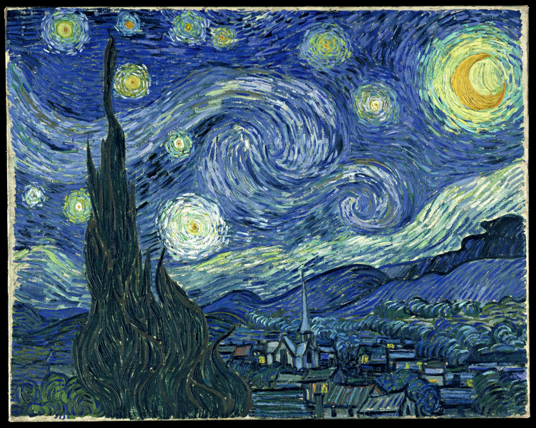
Example 9.1 (Reading in the Starry Night image)

Consider the painting The Starry Night. The original colours are shown in Figure 9.1.

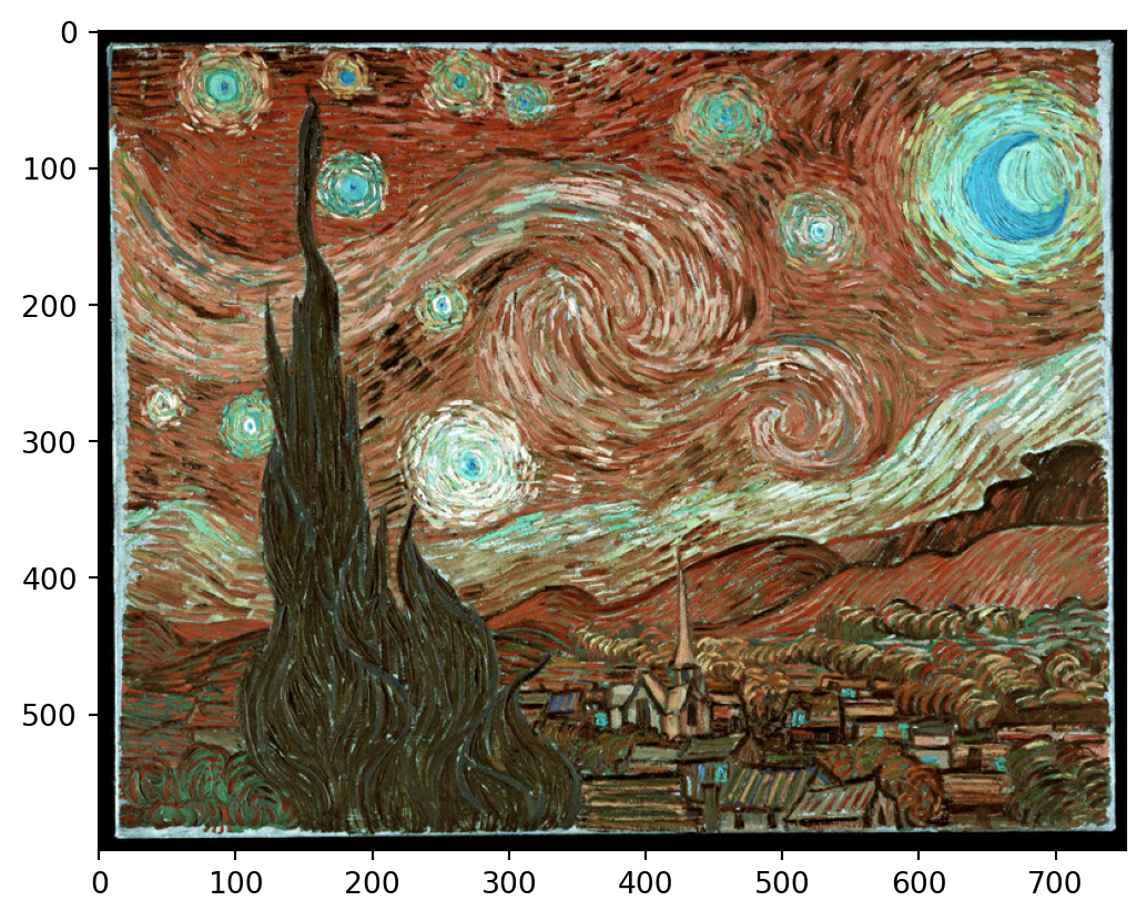
Figure 9.1: Starry Night original colours

However, if we use cv2 to read the image before displaying, the colours will be reversed (see Figure 9.2).

starry_night = cv2.imread('data/starry_night.jpg')
# Reversed (not correct)
plt.imshow(starry_night);

Figure 9.2: Starry Night reversed colour channels

Note

Instead of reading the image file with cv2 and then using matplotlib, we can display the image with cv2 as well. The following code should open up The Starry Night image in a new window on your computer. Press q to close the window.

# plotting with cv2.imshow returns the correct colours.
# Hit any key on the keyboard to close window (do not hit the "X" button)

cv2.imshow('Starry Night', starry_night)
cv2.waitKey()
cv2.destroyWindow('Starry Night')

Ensure that the above works for you, because we are going to be using this approach (instead of matplotlib) to display the capture from your laptop camera in the later sections of this chapter.

Image Transformations

Computer vision models can be sensitive to lighting, angle of capture, and to extraneous objects in the image. Hence it is best to process the image before applying the model; this will typically result in more reliable performance. In this subsection, we demonstrate a few common image processing steps.

Example 9.2 (Common image transformations)

We are going to apply four common transformations to the Starry Night image:

First, we are going to convert the colorspace to grayscale. Several computer vision techniques work only on grayscale images, so this is a common step to be aware of. Take note that grayscale images are numpy arrays with shape \(R \times C\), whereas RGB/BGR images are stored as arrays with shape \(R \times C \times 3\).

# create grayscale version of image
sn_grayscale = cv2.cvtColor(starry_night, cv2.COLOR_BGR2GRAY)

Second, we shall demonstrate how to translate an image. In the code for this procedure, take note that the origin (ie. the (0,0) coordinate) is at the top-left corner. The x-values increase to the right from there until the number of columns; y-values increase downward from there until the number of rows.

rows,cols = starry_night.shape[:2]

# Create RGB version of translated image, moved 400 pixels to the right, and
# 100 pixels down. The translation matrix must be of the form:
# [ [1, 0, x-distance],
#   [0, 1, y-distance]]
M = np.float32([[1, 0, 400],[0, 1, 100]]) # Translation matrix
sn_translate = cv2.warpAffine(starry_night, M, (cols, rows))
sn_translate_rgb = cv2.cvtColor(sn_translate, cv2.COLOR_BGR2RGB)

The third code snippet demonstrates how to rotate an image. For this, and the previous step, we require a transformation matrix, that we then apply to the image using cv2.warpAffine.

# Create RGB version of image, rotated 30 degrees anti-clockwise, about it's 
# centre.
rotation_matrix = cv2.getRotationMatrix2D((0.5*cols, 0.5*rows), 30, 1)
sn_rotated = cv2.warpAffine(starry_night, rotation_matrix, (cols, rows))
sn_rotated_rgb = cv2.cvtColor(sn_rotated, cv2.COLOR_BGR2RGB)

Finally, we show how an image can be resized (scaled up or down) using opencv. When an image is made larger, the pixels need to be interpolated to fill up the gaps; this can be done using a linear or cubic interpolation.

# Resize the image by 20% in each direction, with cubic interpolation.
sn_resized = cv2.resize(starry_night, None,fx=1.2, fy=1.2, 
                        interpolation = cv2.INTER_CUBIC)
sn_resized_rgb = cv2.cvtColor(sn_resized, cv2.COLOR_BGR2RGB)
# Uncomment this line to save the new image and compare with the original.
# cv2.imwrite('data/test_sn.jpg', sn_resized)

Figure Figure 9.3 displays the four transformed images using matplotlib. Take note of the axes dimensions for the resized image; although the displayed image appears to be the same size as the others, it is not, due to the resizing.

There are several other image processing steps that can be very helpful to know about. These include smoothing, thresholding, and morphological operations such as erosion, dilation, opening and closing. Please refer to linked pages on the opencv documentation website for examples and details.

Working with Masks

When working in a computer vision project, we often need to extract parts of the image to work with, or to modify. This is typically done using masks. Masks are black-and-white images that identify the foreground (white) and the background (black). This is also sometimes referred to as binary thresholding.

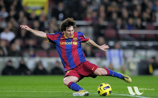
Let us work with the following image of Lionel Messi (Figure 9.4), and see how we can use masks and colour selection to outline the ball.

Example 9.3 (Creating a mask for the football)

After reading the image into Python, we are going to use a colour picker to identify the colour of the ball. The following website provides a useful tool for us to upload an image, and isolate the RGB representaion of the colour we wish to pick out: https://redketchup.io/color-picker

Using this website, we learn that the RGB representation we want is \((244, 251, 95)\). It should be clear that there is a range of values corresponding to the yellow of the ball. To accommodate this range, we convert the colour representation to HSV (Hue-Saturation-Value), using a function from cv2.

# R=244, G=251, B=95
cv2.cvtColor(np.uint8([[[95, 251, 244 ]]]), cv2.COLOR_BGR2HSV)

array([[[ 31, 158, 251]]], dtype=uint8)

The resulting tuple corresponds to the HSV representation of the ball’s colour. The first coordinate corresponds to the hue. We use it to set a range of values to pick up in the image.

messi = cv2.imread('data/messi5.jpg')
hsv = cv2.cvtColor(messi, cv2.COLOR_BGR2HSV)

# define range of yellow color in HSV, using H=31, S=158, V=251 as the reference.
lower_yellow = np.array([21,  100, 100])
upper_yellow = np.array([41, 255, 255])

The final line of code to create the mask is the following.

# Threshold the HSV image to get only blue colors
mask1 = cv2.inRange(hsv, lower_yellow, upper_yellow)
plt.imshow(mask1, cmap='gray');

Figure 9.5: Mask for football, and other yellow segments.

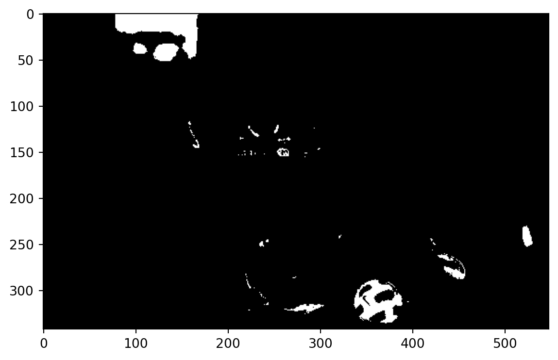
Compare the black-and-white image in Figure 9.5 with the original one in Figure 9.4. The white regions below correspond to yellow coloured sections in the original image. The white pixels take the value 255, while the black pixels are 0.

Just before we close this example, we are going to modify the numpy array corresponding to this mask, to encompass the whole ball, not just the yellow segments.

mask1[:, :330] = 0
mask1[:, 405:] = 0

The next section of code identifies contours around the ball region, computes the convex hull around these points and then draws this on the original image (see Figure 9.6).

#im2, contours= cv2.findContours(mask1, cv2.RETR_TREE, cv2.CHAIN_APPROX_SIMPLE)

contours, _ = cv2.findContours(mask1, cv2.RETR_EXTERNAL, cv2.CHAIN_APPROX_SIMPLE)

largest_contour = max(contours, key=cv2.contourArea)
hull = cv2.convexHull(largest_contour)
cv2.drawContours(messi, [hull], -1, (0, 0, 255), thickness=2)

plt.imshow(cv2.cvtColor(messi, cv2.COLOR_BGR2RGB));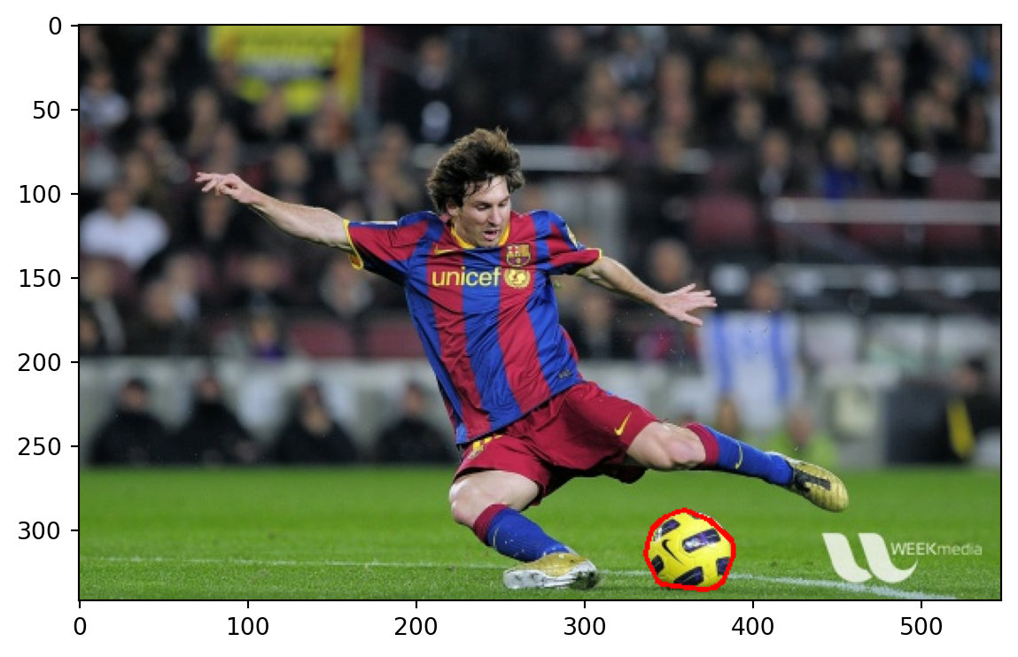

Figure 9.6: Lionel Messi with outline of ball

Modifying Perspective of Images

There are situations where we need to transform the perspective of an image, in order to identify objects better, or to perform OCR better. To do so, we need to provide a map of four points from the original image (in the same plane), and the corresponding four points in the transformed image. At its heart, this is still a transformation, just like a rotation or a translation, but the transformation will not preserve lengths and angles. Here are a couple of examples.

Example 9.4 (Sudoku perspective transform)

Here is an example of transforming the perspective of a sudoku board from a newspaper. The coordinates that result in the red quadrilateral in Figure 9.7 were obtained by manual inspection; this process typically requires a little trial and error.

sudoku = cv2.imread('data/sudoku.png')

# Coordinates of original reference points
pts1 = np.float32([[73,85], [350, 88], [355, 360], [48, 357]])

# Create a polygon (clockwise) from reference points.
pts = np.array(pts1, np.int32)
img2 = cv2.polylines(sudoku, [pts], True, (255, 0, 0), 2 )
plt.imshow(img2);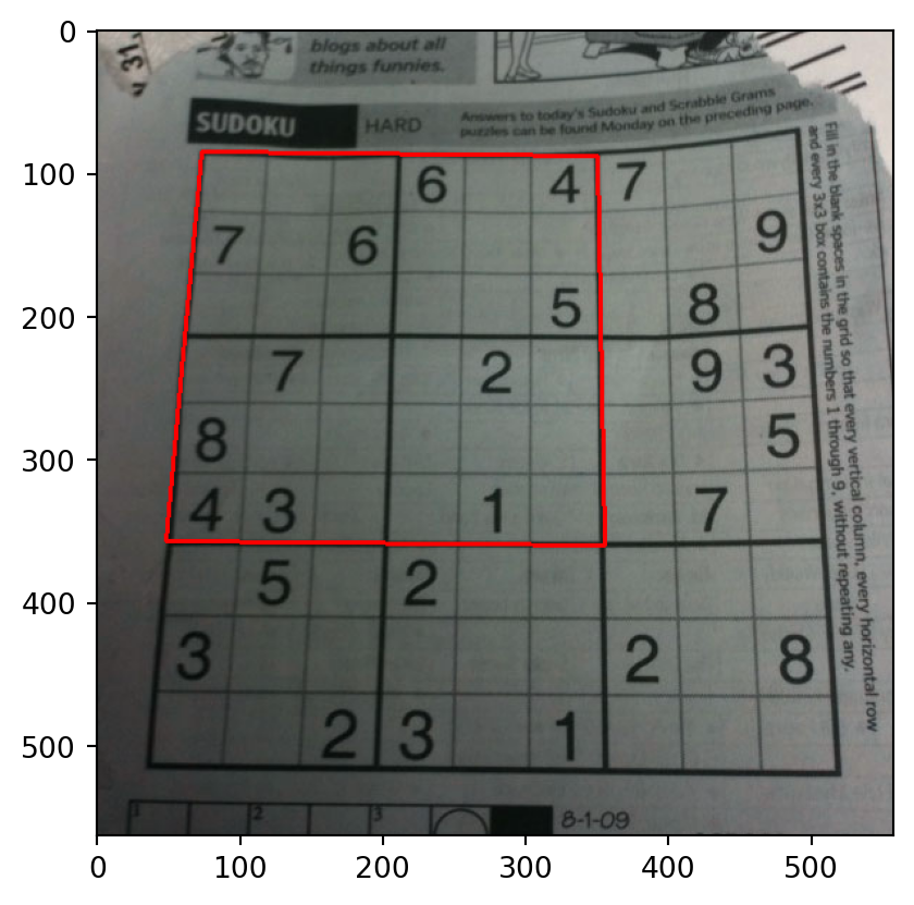

The critical functions are cv2.getPerspectiveTransform and cv2.warpPerspective. The output of the transformed figure is shown on the right of Figure 9.8. It would be much easier to perform OCR on the figure on the right.

# destination coordinates of original reference points.
pts2 = np.float32([[0,0],[300,0],[300,300],[0,300]])
M = cv2.getPerspectiveTransform(pts1,pts2)
sudoku_dst = cv2.warpPerspective(sudoku ,M,(300,300))
 
plt.subplot(121),plt.imshow(sudoku),plt.title('Input')
plt.subplot(122),plt.imshow(sudoku_dst),plt.title('Output');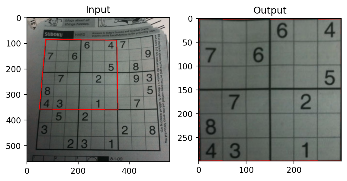

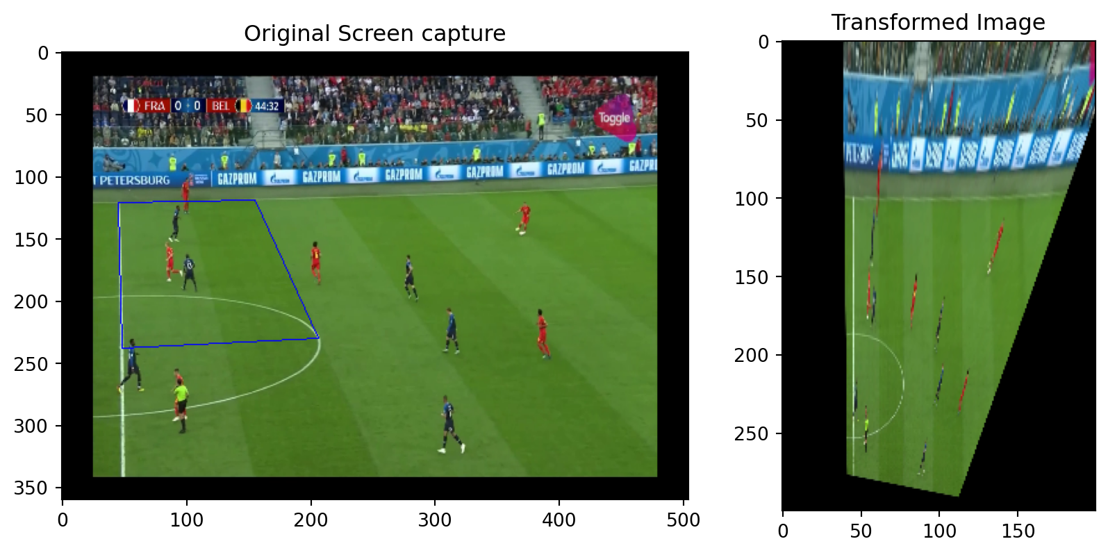
Figure 9.8: Sudoku original and transformed

For our second example, we turn to a screen capture of a football game telecast. Our goal is to switch the view from that in Figure 9.9 to a top-down view of the field.

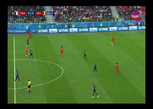
Figure 9.9: Football match screen capture

Example 9.5 (Football screen capture)

Once again, it should be emphasised that the coordinates to be chosen require some trial and error.

football1 = cv2.imread('data/football1.png')
pts1 = np.float32([[45,121],[48,238],[206,230], [155,118]])
pts2 = np.float32([[45,100], [45,220], [77,220], [77,100]])

M = cv2.getPerspectiveTransform(pts1,pts2)
dst = cv2.warpPerspective(football1, M, (504, 360))

pts = np.array([[45,121],[48,238],[206,230], [155,119]], np.int32)
pts = pts.reshape((-1,1,2))
img2 = cv2.polylines(football1, [pts], True, (255, 0, 0), 1 )

From Figure 9.10, it should be clear that only the plane of the field is transformed. The crowd in the stands, and even the players on the field, are in a different 2-D plane, and hence appear distorted.

9.3 Edge Detection

In an image, an edge could refer to a discontinuity in surface colour, surface depth, surface direction, or illumination (see Figure 9.11).

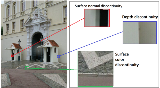
Figure 9.11: Examples of edges in images, taken from Stanford notes.

Almost all edge detection methods rely on computation of the gradient of pixel values. If there is a contiguous sharp change along a line, it is indicative of an edge.

Example 9.6 (Sudoku edge detection)

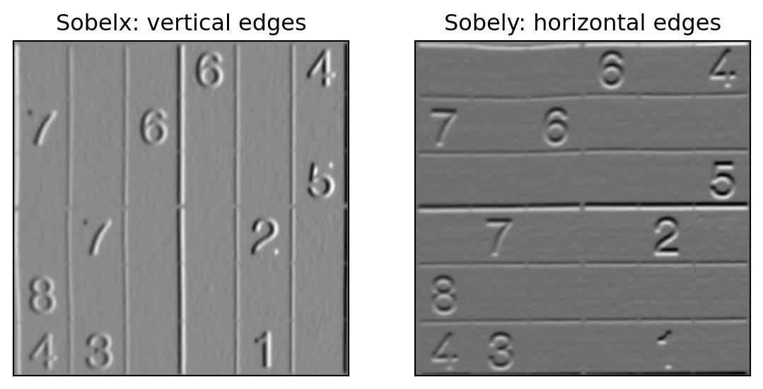
The Sobel edge detection technique is one of the most straigtforward to understand. It can be used to detect vertical or horizontal edges. Let us apply this technique to the perspective-transformed Sudoku image from Example 9.4.

Edge detection is almost always performed on the grayscale version of an image. In the code segment below, sobelx and sobely now contain the vertical (in the x-direction) and the horizontal (in the y-direction) edges.

dst_gray = cv2.cvtColor(sudoku_dst, cv2.COLOR_BGR2GRAY)
sobelx = cv2.Sobel(dst_gray, cv2.CV_64F, 1, 0,ksize=5)
sobely = cv2.Sobel(dst_gray, cv2.CV_64F, 0, 1,ksize=5)

Figure 9.12 displays the resulting edges from the Sobel technique.

plt.subplot(1,2,1),plt.imshow(sobelx, cmap = 'gray')
plt.title('Sobelx: vertical edges'), plt.xticks([]), plt.yticks([])
plt.subplot(1,2,2),plt.imshow(sobely, cmap = 'gray')
plt.title('Sobely: horizontal edges'), plt.xticks([]), plt.yticks([]);

Figure 9.12: Sudoku vertical and horizontal edges

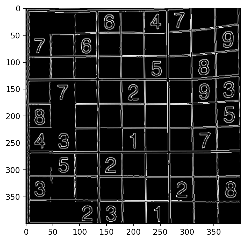
Most edges in real-life images are not as perfect as those in a Sudoku table. The Canny edge detection technique relies on a multi-step approach to identify edges in any and all directions. Just like the Sobel approach, the Canny edge detection technique identifies pixels where the gradient changes sharply with edges. However, in the next step, based on two input parameters provided by the user, weak edges are dropped, and strong edges are retained. The ones in the middle are only retained if they are connected to a strong edge.

Example 9.7 (Canny edge detection of ball)

Earlier in Example 9.3, we used the colour of the ball to locate it within the image. In this example, we are going to use Canny edge detection. First, take a look at the application of the algorithm to the grayscale version of the image, in Figure 9.13. Play around with the two parameters (150 and 200) to see the effect on the number of edges produced.

messi_gray = cv2.cvtColor(messi, cv2.COLOR_BGR2GRAY)
messi_canny_edge = cv2.Canny(messi_gray, 150, 200)
plt.imshow(messi_canny_edge, cmap='gray')

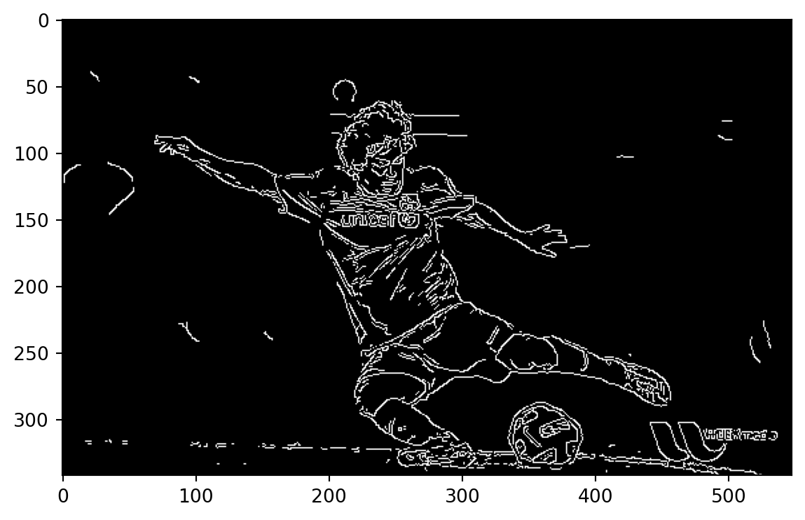
The next step involves the use of Hough transforms. When applied to edges, this transform can be used to pick out lines that follow any parametric form, e.g. lines, quadratic curves, ellipses and circles. Since we know the ball is a circle, we are going to use the Hough transform to pick it out from the edge map.

blurred = cv2.GaussianBlur(messi_gray, (9, 9), 2)

circles = cv2.HoughCircles(blurred, cv2.HOUGH_GRADIENT, dp=1,
                            minDist=50,
                            param1=50,
                            param2=22,      # low threshold to start, 22 works best
                            minRadius=18,
                            maxRadius=38)

print(circles)

[[[297.5 169.5  35.2]
  [361.5 313.5  28.4]
  [231.5  96.5  20.5]]]

Three circles have been located in the image! Figure 9.14 marks out all three circles found.

Note

Can you think of contextual information you can use to rule out the erroneous balls?

circles_rounded = np.uint16(np.around(circles))
for i, c in enumerate(circles_rounded[0, :]): 
    cv2.circle(messi, (c[0], c[1]), c[2], (0, 255, 0), 2)     # circle 
    cv2.putText(messi, str(i), (c[0], c[1]),                  # label each one 
                cv2.FONT_HERSHEY_SIMPLEX, 0.6, (255,255,0), 2)

plt.imshow(cv2.cvtColor(messi, cv2.COLOR_BGR2RGB))
plt.title('Detected circles (numbered)');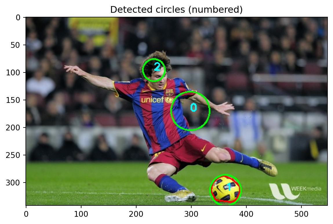

Figure 9.14: Circles detected with Hough transform

9.4 Computer Vision Demonstrations

Just as we observed there are numerous NLP tasks, the field of computer vision has made great strides in several tasks. Among them are:

Object detection
Object classification
Object tracking
Face detection
Pose estimation
QR/Bar code detection
Text detection/extraction

Almost all the models that perform well in the above tasks are deep learning models. In the next few sections, we are going to practice running/configuring some of the above models. Although these models are already trained, it is a little tricky to find the resources and parameters to get them up and running.

Before beginning, download the following three repositories and unzip them into the same folder:

For instance, your folder structure may now be :

|-01-lecture.ipynb
|-... other files
|-opencv/
|-opencv_extra/
|-opencv_zoo/

opencv: This repository contains example images and videos, and configuration files for several models. It also contains the routines to download models.
opencv_extra: This contains more configuration details for the models.
opencv_zoo: This contains a smaller range of models, along with the model weights.

Models from OpenCV Repository

First, we demonstrate how to download models using the script in opencv. Open up a terminal, activate your virtual environment and navigate into opencv/samples/dnn.

Next, check inside models.yml for the model that you intend to use. The list of models available are:

Model Type	Model Name
Object Detection	opencv_fd
Object Detection	yolov8x
Object Detection	yolov8s
Object Detection	yolov8n
Object Detection	yolov8m
Object Detection	yolov8l
Object Detection	yolov5l
Object Detection	yolov4
Object Detection	yolov4-tiny
Object Detection	yolov3
Object Detection	tiny-yolo-voc
Object Detection	yolov8
Object Detection	ssd_caffe
Object Detection	ssd_tf
Object Detection	faster_rcnn_tf
Image Classification	squeezenet
Image Classification	googlenet
Semantic Segmentation	enet
Semantic Segmentation	fcn8s
Semantic Segmentation	fcnresnet101

For this demonstration, we shall aim to download and run the GOOGLENET image classification model. Run the following command to download the model weights for GOOGLENET:

python .\download_models.py --save_dir GOOGLENET googlenet

Apart from listing all the models available for download, models.yml also contains the precise configuration settings to run this particular model. For full reference, here is the section corresponding to GOOGLENET:

# Googlenet from https://github.com/BVLC/caffe/tree/master/models/bvlc_googlenet
googlenet:
  load_info:
    url: "http://dl.caffe.berkeleyvision.org/bvlc_googlenet.caffemodel"
    sha1: "405fc5acd08a3bb12de8ee5e23a96bec22f08204"
  model: "bvlc_googlenet.caffemodel"
  config: "bvlc_googlenet.prototxt"
  mean: [104, 117, 123]
  scale: 1.0
  width: 224
  height: 224
  rgb: false
  classes: "classification_classes_ILSVRC2012.txt"
  sample: "classification"

The important parameters to take note are:

model: Refers to the file containing the model weights (which we just downloaded)
config: Configuration parameters. This file is usually present in the opencv_extra repository.
mean, scale, width, height, rgb: Arguments that need to be included when calling the python script object_detection.py.
sample: The python script to call, to demonstrate the use of this model.
classes: GOOGLENET is an object classification model. The specified file here contains the labels to be used. The file is present in the opencv/samples/data/dnn directory.

The final step is to call the python script that demonstrates the use of this model. You may have to modify the paths to the image files to match those on your laptop, but you should then see the labelled image, similar to Figure 9.15.

python classification.py --model GOOGLENET/405fc5acd08a3bb12de8ee5e23a96bec22f08204/bvlc_googlenet.caffemodel \
--config /home/viknesh/NUS/coursesTaught/ind5003-book/opencv_extra/testdata/dnn/bvlc_googlenet.prototxt \
--width 224 --height 224 --classes ../data/dnn/classification_classes_ILSVRC2012.txt \
--mean 104 117 123 --input /home/viknesh/NUS/coursesTaught/ind5003-book/data/cars.jpg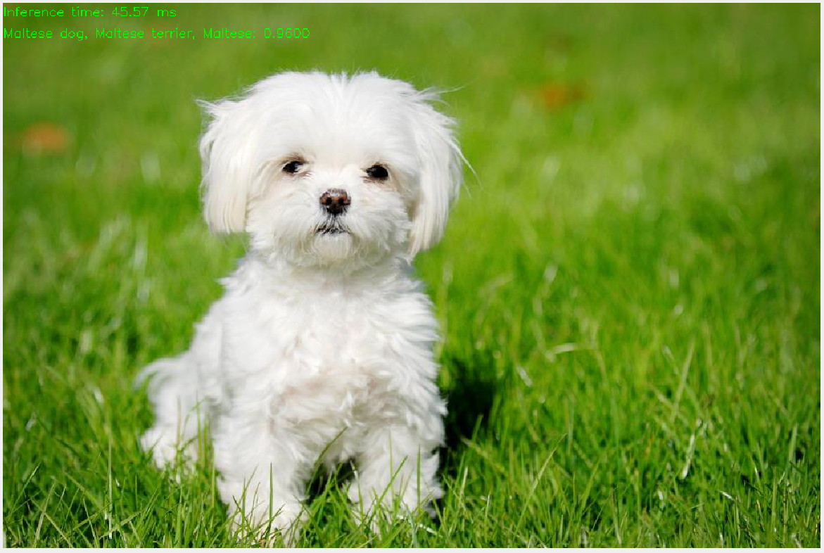

Utilising the sample models can be a little tricky, because one has to search for the right files to use, and the precise configuration to use, but it is an useful step in learning about the capabilities of vision models.

Models from OpenCV Model Zoo

The openCV model zoo contains model weights that can be used directly. There is no need for any further downloads. Open up a terminal, activate your virtual environment, and navigate to the opencv_zoo/models/face_detection_yunet/ folder. Then run the following command:

python demo.py

9.5 Summary

Our chapter is a very brief introduction to vision models. I encourage you to explore the sample models to understand the capabilities and the various tasks they have been trained for.

In real-life projects, there will undoubtedly be a large amount of pre-processing required before the models can be applied to each image. While the initial section of the chapter touches on these steps, you should read up on the details, and follow-up with the websites to become more adept at image manipulation and processing with opencv.

9.6 References

Opencv documentation

Python tutorials
Changing colour spaces
Background subtraction
Opencv bootcamp: This is a very useful course on opencv techniques. It will also provide you several more notebooks with template code for object tracking, etc.

Books

A very comprehensive book on vision techniques is by Szeliski (2022). An online version can be found here: Computer Vision: Applications and Algorithms

Github repositories

9.7 Exercises

In Section 9.4.1, we downloaded and used the GOOGLENET model. Follow the procedure to download and apply the YOLOv4-tiny model to the same image.
Use the VIT (vision transformer tracker) to track one of players in this video. The tracker can be found in the opencv model zoo.
Use Canny edge detection, and then a perspective transform, to create Figure 9.16, starting from the Sudoku image:

Rotate The Starry Night image 45 degrees clockwise about the top-left corner of the image. Display the result using matplotlib, ensuring the colours appear correct.
Use the colour picker to isolate the blue regions of Messi’s Barcelona jersey.